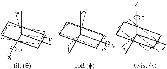

Three angular parameters (tilt, roll and twist) define the position and direction of one base pair relative to the next. The tilt angle (theta) is defined as a rotation about the X axis, the roll angle (phi) is about the Y axis and the twist angle (tau) is rotation about the Z axis. For instance, defining these angles between two base pairs in a stretch of perfectly straight B-form DNA would be: tilt=0, roll=0 and twist=36 (assuming a helical repeat of exactly 10 bp).

Thus, a single DNA chain of N base pairs in length can be described by 3*(N-1) parameters defining the tilt, roll and twist angles between each base pair, assuming the first base pair has a known fixed position.
The sequence.in file (which can be generated by the CYCLIZE PERL subroutines) contains six values per base pair step describing the chain's tilt, tilt_flex, roll, roll_flex, twist and twist_flex. Each of these values is in degree units. The flexibility parameters describes the range of the thermally induced gaussian fluctuations for each of the base pair's tilt, roll and twist angles.
The program reads this information, and chops the chain into two partitions (ie: a 156 nt DNA becomes two partitions from 1-78 bps and 79-156 bps). The Monte Carlo routine "generate_chain" (found in cyclize_lib.c) is then called a "number of half-chain" times for each partition. The half-chains generated for the partitions are then stored in binary form in the files "chain_1.dat" and "chain_2.dat".
Finally, a report is generated called 'generate_chains.header", which contains gobs of information on how the chain generation was performed.
For instance, if you set tilt=0, roll=0 and twist=36, this is defining that the next bp is, on average, planar with the previous bp (tilt=0 and roll=0) but has a 36 degree twist about the Z-axis (ie: B-form DNA has an approx 36 degree twist from one base pair to the next).
Three functions that return random numbers with a gaussian distribution (a normal distribution, in stats speak) have been coded into CYCLIZE and all can be found in the source code file named "math_routines.c". The first function is called gauss and calculates a normal distribution by averaging 12 random numbers from 0-1, this routine is VERY slow, due to the large number of calls to the RNGs. The second is called gauss_box_muller and is from the Numerical Recipies people using the Box-Muller algorithm (see page 289 of "Numerical Recipies in C", 2nd ed.). The third routine is called gauss_dev2 was found on the internet somewhere. The gauss_box_muller routines makes only two calles to the RNG on average (is this always true?) and is the fastest of the routines and is thus what is used by default for CYCLIZE.

Each distribution function is stored seperately every 10% of the calculation, allowing for the calculation of the "summed" distribution function and the standard deviation of each point in this summed distribution function. All discussions below are concerning this "summed" distribution function.
The radial distribution function is stored as an integer array in which each position (or "bin" in stats speak) of the array represents an additional 1 angstrom end-to-end distance for the chain. Thus, the 6th bin of the distribution array will count the number of chains with an end-to-end distance between 5.0-6.0 angstroms.
After the simulation is finished, each bin of the distribution array is converted to a "molarity" distribution function, rather than a "counting" distribution function. This is accomplished by dividing the "fractional moles of chains" by the "shell volume". The best way to explain this is to demonstrate the actual formula.
Variable definitions
f           = fractional # of chains in the current bin
chains_bin  = number of chains in the current bin
nR_analyzed = number of chains stored in all bins
moles_chain = fractional moles of a chain in the current bin
volume_bin  = volume of the current bin
Na          = Avagadro's number
R1          = smallest radius allowed in the current bin
R2          = largest radius allowed in the current bin
W_bin       = "molarity" of the current bin
Equations used:
f          = chains_bin / nR_analyzed
moles_bin  = f / Na
volume_bin = 4/3 * PI * [R2^3 - R1^3]
W_bin      = moles_bin / volume_bin
The final radial "molarity" distribution function is fit by a even powered quadratic function: Y=A + BX^2 + CX^4 using Single Value Decomposition. Only the first 30% of the function is used in the fitting, since we ultimately only want to know what the Y intercept is, there is no need to fit points far from X=0.
The axial distribution function is fit by a even powered quadratic function: Y=A + BX^2 + CX^4 using Single Value Decomposition.
The torsional distribution function is fit by a gaussian function: Y=A * exp[ - ( (x-B)/(1.414*C) )^2 ] using the Leveberg-Marquardt methodology.